VOYAGER

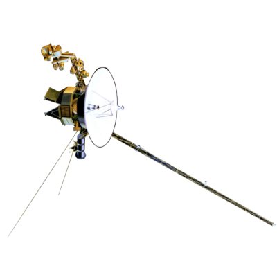
Voyager LECP Data Analysis Handbook

 

Instrument Modeling Reports

 

An Analysis of the Performance of the Magnetic Deflection System
 in the Voyager Low Energy Charged Particle Experiment

 

by Sheela Shodhan

 

Chapter 5. Calculations and Results

 

5.1 Calculations

 

The geometric factor G of a detector for a particular energy is the sum over all the sampling areas of the detector of the product of the sampling area of the detector and the solid angle spanned by the open trajectories that connect the sampling area and the open aperture, i.e.:

 

G = n  å i = 1  ΔAiΔΩi

 

where n is total number of sampling areas on the detector,

 

ΔA_i is the area of the ith. element on the detector,

 

ΔΩ_i is the solid angle spanned by the open trajectories

 

≈ Σ_{j = 1}^npasΔθ_jΔΦ_j sin( θ_j+[(Δθ_j)/2])

 

Δθ,ΔΦ are the intervals at which the polar and the azimuthal angles are scanned respectively and npas is the number of trajectories connecting ΔA_i and the open aperture.

 

5.1.1 Determination of DAi

 

Each of the circular detector surfaces is divided into several sampling areas ΔA_i. Each one of these circular surfaces is fitted into a square which is then further divided into smaller squares. The centres of each of these smaller squares which fall within the circular detectors have been considered as to sample that particular area element. Those squares that contain the centre point but are cut off by the circular boundary of the detector have been approximated as trapezoids.

 

Then starting from a particular center point on the detector, for a particular energy, the solid angle is determined.

 

 

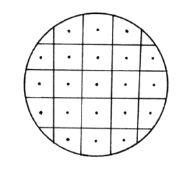
Figure 5.1. The detector surface divided into several sampling areas. The dotted points are the initial points of the trajectory.

 

5.1.2 Determination of the solid angle

 

For a given energy, starting from a particular point on the detector and with a particular set of polar and azimuthal angles, the motion of this particle is observed inside the sensor subsystem. The coordinates of these points are included in Appendix D. The equations of motion:

 

dX/dt = V

M dV/dt = q/c V × B

 

are solved by Hamming's modified double precision Predictor-Corrector method in a "time reversed sense." "Time reversed sense" because the starting point on the detector surface in this calculation is the end-point of the real particle. At every stage of the trajectory calculation the fate of the particle is determined as discussed later. If this particle's trajectory passes through the open aperture of the sensor subsystem then it is considered as escaped. The polar and the azimuthal angles at the aperture are computed and npas is incremented by one. However, if the particle hits any of the surfaces of the sensor subsystem then it is considered lost and thus ignored since the real particle would also not be able to hit this point on the detector. Then a new set of polar and azimuthal angles is chosen and this process is repeated. Thus, polar and azimuthal are scanned at specific intervals to determine whether the particle escapes or not. A specific range of these for which the particles escape the sensor subsystem forms the set of trajectories that connect the sampling area and the open aperture. Then the solid angle spanned by this set of trajectories is computed using the above equation.

 

5.1.3 Determination of the fate of the particle

 

Given the line-segment formed by the points (x_i,y_i,z_i) and (x_i+1,y_i+1,z_i+1) of the trajectory to determine whether the particle is lost or not, the process is as follows:

 

1. Knowing the coordinates of each of the vertices of the plane polygon, the equations of the planes for all the modelled polygons that comprise the sensor subsystem are determined.
2. Given the line-segment of the trajectory, find whether the line formed by these two points is parallel to a given plane or not.
3. If the line is not parallel then find the intersection point of this line and the plane.
4. Find whether this intersection point belongs to the line segment bounded by (x_i,y_i,z_i) and (x_i+1,y_i+1,z_i+1) or not. If it does not belong to the line segment then the particle has not reached the plane yet and so it is not lost.
5. However, if the intersection point belongs to the line-segment, then determine whether this point lies on the surface of the polygon (finite region of the plane) or not. For all surfaces, except the apertures of the housings of the detectors, deflection system and the opening aperture of the aperture cone, if the particle lies on the surface of the plane polygon then it is considered to be lost, otherwise not. However, if it lies outside the surfaces of the apertures of the housings, deflection system and the aperture cone, it is considered to be lost.

 

For each of the steps above from (1) to (5) the relevant equations used are included in Appendix C.

 

In this way, the trajectory calculation continues until a decision is made as to whether the particle hits any of the surfaces and is lost or it passes through the opening aperture and escapes.

 

 

5.2 Discussion of the Results

 

Since at every stage in the particle's trajectory its curvature is determined by the local relation,

 

r = mcv/Bq    (in c.g.s. units)

 

the deflection of the low energy electrons should be more than that of the high energy ones. This explains the fact that the Beta detector, which is closer to the opening aperture than Gamma, primarily collects low energy electrons while the Gamma detector collects higher energy electrons.

 

On examining the trajectories of the particles of different energies emanating either from the Beta detector or the Gamma detector, we do observe that the low energy electrons are indeed deflected more than the high energy ones. This also manifests itself in the shift of the azimuthal angles for which the particles escape, from lower angles to higher angles, as the energy increases. For example, for the energy E=480 keV the range of azimuthal angles for a point on the Gamma detector is 167 to 227 deg. while for the same point for energy E=720 keV the range has shifted to 181 to 228 deg. 

 

Also, for a particular energy, due to the inhomogeneity of the magnetic field, the curvature of the trajectory of the particle depends upon its position in the deflection system. In this time reversed calculation, the particles entering the deflection system into the region where the field is higher have higher curvatures (less radii) whilst those particles that enter into the region of lower field have lower curvatures (high radii).

 

Together with this field inhomogeneity which shapes the trajectory of the particles, the surfaces of the sensor subsystem restrict the values of the angles for which the particles escape to a finite range instead of all the allowable values.

 

Besides, we also expect the symmetry about the z = 0.0 plane in the magnetic field and in the modelled sensor subsystem, to be reflected in the angular distributions of the escaping particles at the detectors and at the apertures.

 

1. The particles that escape from a point on the z = 0.0 plane of the detector should have an even distribution in the polar angle (theta) about θ = 90 deg, i.e. if the particle passes for a polar angle θ = 85 deg then there should be corresponding pass for the angle θ = 95 deg also. This symmetry about θ = 90 deg is well demonstrated by the plots of angular distribution (see figures 5.8 to 5.13) for particles of various energies emanating from the point z = 0.0 of the detectors.
2. Also, the number of particles that escape from the two points situated on either side of z = 0.0 plane of the detector should be the same. This is presented in the plots (see figures 5.14 to 5.16) that show the angular distribution of the escaping particles. Although these particles have the same range of the azimuthal angles, the distribution of the polar angles about θ = 90 deg is not symmetric. This is because while scanning over θ < 90 deg it hits one of the side surfaces sooner or later than the corresponding side for scans θ > 90 deg depending upon its position about the z = 0.0 plane.

 

The above observations support the validity and the correctness of the magnetic field model.

 

5.2.1 Variation of the geometric factors with energy

 

DETECTOR	ENERGY keV	GEOMETRIC FACTOR cm2 sr
Beta	40	0.010177
	80	0.025129
	160	0.026672
	320	0.003406
	480	0.000803
Gamma	250	0.019426
	500	0.038626
	720	0.024262
	1440	0.005594
	2880	0.000992

 

Table 5.1. Geometric factors for different energies for the Beta and the Gamma detectors

 

5.2.2 Tables of the number of particles that pass

 

 

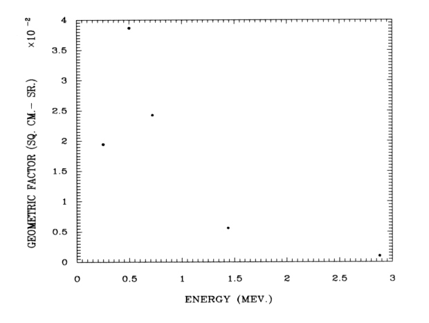
Figure 5.2. Variation of the geometric factors with energy for the Gamma detector.

 

 

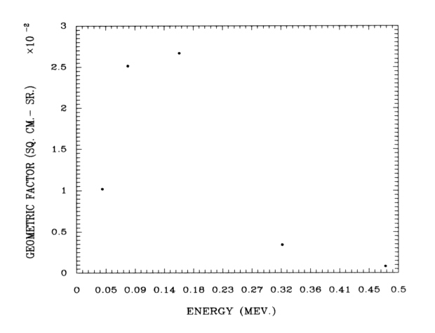
Figure 5.3. Variation of the geometric factors with energy for the Beta detector.

 

 

Figure 5.4. Points on the Gamma detector which are the initial points of the trajectories.

 

	2	4	6	8	10
2		499	526	499
4	498	528	531	528	498
6	528	557	576	557	528
8	552	576	576	576	552
10		568	564	568

 

Table 5.2. Number of particles that pass for different points on the Gamma detector for E=500 keV. Note: The scanning intervals Δθ, ΔΦ = 2 deg.

 

	2	4	6	8	10
2		245	265	245
4	286	301	314	301	286
6	331	346	1402*	346	331
8	361	387	379	387	361
10		419	404	419

 

Table 5.3. Number of particles that pass for different points on the Gamma detector for E=720 keV. Note: The scanning intervals Δθ, ΔΦ = 1 deg for point marked by *, for all others, Δθ,ΔΦ = 2 deg.

 

	2	4	6	8	10
2		32	37	32
4	31	54	64	54	31
6	60	83	350*	83	60
8	93	106	114	106	93
10		125	137	125

 

Table 5.4. Number of particles that pass for different points on the Gamma detector for E=1440 keV. Note: The scanning intervals Dθ, ΔΦ = 2 deg and for points marked *, Dθ, ΔΦ = 2 deg.

 

	2	4	6	8	10
2		0	10	0
4	0	13	37	13	0
6	10	53	74	53	10
8	45	93	120	93	45
10		151	162	151

 

Table 5.5. Number of particles that pass for different points on the Gamma detector for E=2880 keV. Note: The scanning intervals Δθ, ΔΦ = 1 deg.

 

 

Figure 5.5. Points on the Beta detector which are the initial points of the trajectories.

 

	2	4	6	8	10
2		124	140	124
4	54*	67*	70*	67*	54*
6	107	129	142	129	107
8	97	123	66*	123	97
10		100	54*	100

 

Table 5.6. Number of particles that pass for different points on the Beta detector for E=40 keV. Note: The scanning intervals Δθ = 2 deg. For points marked by *, ΔΦ = 4 deg, for others ΔΦ = 2 deg.

 

	2	4	6	8	10
2		131	137	131
4	258*	292*	150	292*	258*
6	142	155	164	155	142
8	145	160	164	160	145
10		163	165	163

 

Table 5.7. Number of particles that pass for different points on the Beta detector for E=80 keV. Note: The scanning intervals Δθ = 2 deg. For points marked by *, ΔΦ = 2 deg, for others ΔΦ = 4 deg.

 

	2	4	6	8	10
2		140	149	140
4	136	153	168	153	136
6	141	166	172	166	141
8	156	171	176	171	156
10		173	177	173

 

Table 5.8. Number of particles that pass for different points on the Beta detector for E=160 keV. Note: The scanning intervals Δθ = 2 deg. and ΔΦ = 4 deg.

 

	2	4	6	8	10
2		18	28	18
4	11	48	95	48	11
6	72	153	204	153	72
8	198	310	360	310	198
10		532	566	532

 

Table 5.9. Number of particles that pass for different points on the Beta detector for E=320 keV. Note: The scanning intervals Δθ,ΔΦ = 1 deg.

 

	2	4	6	8	10
2		0	0	0
4	0	0	0	0	0
6	0	7	29	7	0
8	16	66	97	66	16
10		158	188	158

 

Table 5.10. Number of particles that pass for different points on the Beta detector for E=480 keV. Note: The scanning intervals Δθ,ΔΦ = 1 deg.

 

Additional Figures:

 

• Figure 5.6. Particle trajectories emanating from the point
  (-0.537177,-0.570312,0.0) of the Gamma detector.
• Figure 5.7. Particle trajectories emanating from the point 
  (-0.718812,-0.09375,0.0) of the Beta detector.
• Figure 5.8. Angular distribution for energy E=720 keV.
• Figure 5.9. Angular distribution for energy E=1440 keV.
• Figure 5.10. Angular distribution for energy E=2880 keV.
• Figure 5.11. Angular distribution for energy E=80 keV.
• Figure 5.12. Angular distribution for energy E=320 keV (at the point 
  (-0.718812,-0.09375,0.0) and at the aperture).
• Figure 5.13. Angular distribution for energy E=480 keV.
• Figure 5.14. Angular distribution for energy E=320 keV (at the point 
  (-0.718812,-0.09375,-0.02384) and at the aperture).
• Figure 5.15. Angular distribution for energy E=320 keV (at the point 
  (-0.718812,-0.09375,0.02384) and at the aperture).
• Figure 5.16. Points on the detector Beta which sample the area.

 

 

Appendix A

 

Return to thesis table of contents. 

Return to Voyager LECP Data Analysis Handbook Table of Contents.
Return to Fundamental Technologies Home Page.

VOYAGER 1 ELAPSED TIME

Days: Hours: Minutes: Seconds

*Since official launch
September 5, 1977, 12:56:00:00 UTC

VOYAGER 2 ELAPSED TIME

Days: Hours: Minutes: Seconds

*Since official launch
August 20, 1977, 14:29:00:00 UTC

QUICK FACTS

RELATED LINKS